Pipelines as Code With Delta Live Tables
It has now been almost a year since Databricks released a new ETL framework under the name Delta Live Tables. With this, the San Francisco-based company is focusing on the strategy of being able to use its existing data platform as a general-purpose tool and is pushing forward with its transformation to a single-source-of-truth.
Since I’ve already been involved with various use cases on the platform for over a year, this didn’t pass me by. And so, over the last few months, I’ve had the opportunity to get to grips with the new ETL framework and various new features of the platform.
Why Another ETL Framework?
Delta Live Tables is based on the idea of the Data Lakehouse. This is an approach that unifies traditional data warehouses with data lakes and provides many benefits. If you’re new to this topic, you might want to check out my previous post in that I explain the concept of the Data Lakehouse in more detail.
Further, Delta Live Tables is a mix of common ETL approaches. These usually come in either low-code or high-code fashion. Make sure to check out my latest post on the benefits of these concepts for data processing. This will give you an idea why Databricks might follow a new strategy for their ETL framework.
Delta Live Tables - a Hybrid?
Pipeline Definition
Most low-code platforms rely on a graphical user interface that can be clicked together by a user, Delta Live Tables relies on code as a pipeline definition. This is simplified by a provided package in such a way that it can also be used by less experienced engineers.
Currently, the programming languages Python and SQL are supported by this. For Python there is the closed source package dlt, which must be imported into each pipeline definition.
import dlt
Otherwise, it is a normal notebook by definition.
Tables and Views
In a Delta Live Tables pipeline definition, besides the ability to write functions, the developer now can define tables or views. These look like ordinary functions, but are provided with a decorator.
@dlt.table
def raw_table():
    return spark.read.csv("s3://my_bucket/my_table.csv")
Besides that, you can specify other metadata for the decorator and even change the location if you don’t want to use the default value from the pipeline configuration. This can be useful if this value should be different depending on the environment.
@dlt.table(
    name="my_table",
    description="This is my table",
    location="s3://raw/my_table"
)
def raw_table():
    return spark.read.csv("s3://raw/my_table.csv")


@dlt.table(
    name="my_table",
    description="This is my table",
    location="s3://raw/my_table"
)
def raw_table():
    return spark.read.csv("s3://raw/my_table.csv")
In the above example, a table is defined that is read from a CSV file. This table is then executed and stored in the specified location. However, it is also possible to define streaming jobs besides such batch jobs, which read from a Kafka topic as in the following example.
@dlt.table(
    name="my_table",
    description="This is my table",
    location="s3://raw/my_table"
)
def raw_table():
    return (
        spark.readStream
             .format("kafka")
             .option("kafka.bootstrap.servers", "server:ip")
             .option("subscribe", "topic1")
             .option("startingOffsets", "latest")
             .load()
    )
A nice and helpful feature is also Auto Loader, a tool with which Databricks offers the possibility to use directories in the cloud as a streaming source. New files are automatically detected and loaded into the pipeline. A checkpoint mechanism ensures that no files are processed twice. However, it is also possible to process all files again if required.
@dlt.table(
    name="my_table",
    description="This is my table",
    location="s3://raw/my_table"
)
def raw_table():
    return (
        spark.readStream
            .format("cloudFiles")
            .option("cloudFiles.format", "csv")
            .load("s3://my_bucket/my_raw_data")
    )
Automatic Orchestration
Now that you have defined some raw or bronze tables, you can continue working
with them directly in Delta Live Tables. For this purpose, there is the
possibility to define further tables based on the previous tables. The tables
are automatically executed in the correct order and also asynchronously.
Alternatively, instead of spark, you can use the command dlt.read for this
purpose. This command reads the table from the Delta Lake and returns it as a
data frame.
@dlt.table
def clean_table():
    return (
        dlt.read("raw_table")
            .select("col1", "col2")
            .withColumn("col3", F.col("col1") + F.col("col2"))
    )
In the same way, you can define the clean or gold layer. Of course, you can also merge several tables from the previous steps. The nice thing about this is that such joins are also displayed in the generated graph.
@dlt.table
    def gold_table():
        return (
            dlt.read("clean_table")
               .join(dlt.read("other_table"), "id")
    )
Data Quality
Another possibility offered by a DLT pipeline definition is to define data quality tests. These can apply to individual columns. The mechanism can be used in three variants:
- expect: expects a certain condition to be met. Otherwise, error statistics are collected and displayed in the pipeline graph.
- expect_or_fail: Expects a specific condition to be met. Otherwise, the table and all tables based on it will be aborted.
-
expect_or_drop: Expects a certain condition that must be met. Otherwise, incorrect values will be removed from the table. However, it will not be aborted.
@dlt.expect_or_fail("name IS NOT NULL") @dlt.table def gold_table(): return ( dlt.read("clean_table") .join(dlt.read("other_table"), "id") .withColumnRenamed("name", "first_name") )
Configuration
Even though the pipeline definition is written in code, it is still necessary to put the pipeline into some kind of container. Delta Live Tables offers a configuration for this, which can be defined when creating a pipeline.
It contains the configuration of the cluster and the mode in which the pipeline is started. For example, you can work in a development mode, where the cluster stays on for a longer time. In production mode, in which the pipeline is to be executed only once, the cluster is shut down again after execution.
The version of Delta Live Tables can be selected here, i.e. the features that are required. For example, data quality tests can only be used in the Advanced version.
Of course, you also have to specify the pipeline definition to be used and the database in which the data is to be stored.
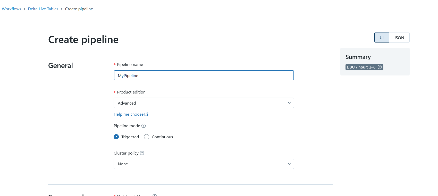 Create a DLT Pipeline, Image source: Fabian Stadler
This means that one pipeline definition can also be used in multiple configurations/pipelines. This is useful if I have multiple development and production environments. It is the same with the choice of database. While I cannot call a DLT pipeline with arguments, it is still possible to do certain things differently in my code in the configuration via Spark parameters. For example, I can specify different file paths for configuration files. Or I can set certain flags that change my pipeline in different places.
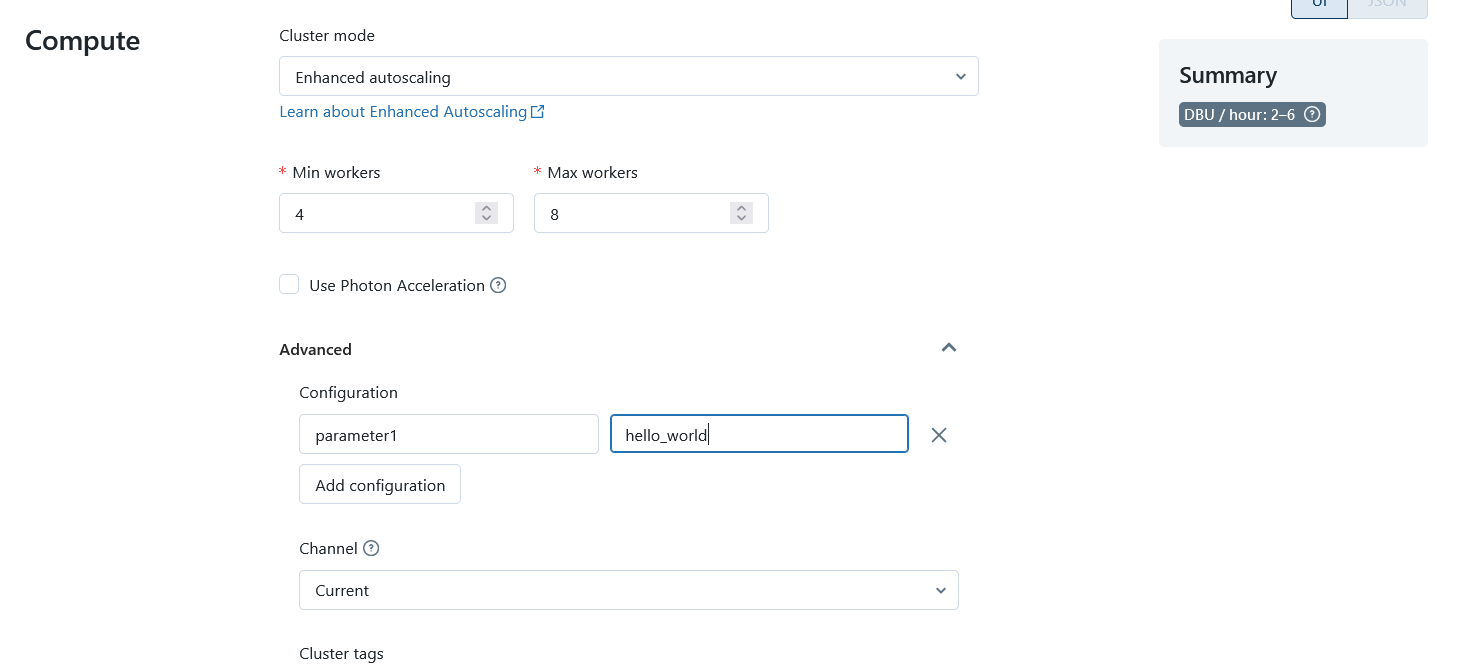 Configure the DLT Cluster, Image source: Fabian Stadler
Execution
After configuring and writing a pipeline, execution is simple with the click of a button. It is also possible to define a schedule or to start the pipeline via the API.
In production mode, a retry is automatically started for errors that DLT considers transient. This can be the case with network problems, for example. However, this does not always work smoothly, which often leads to unnecessary retries.
Visualization
The visualization of the data pipeline is done via so-called DAGs (Directed Acyclic Graphs). These are like the graphical interfaces of low-code platforms, but with some advantages. On the one hand, they are usually easier to read and understand. For another, they can be opened and edited by a code editor. Most low-code platforms do not offer this possibility. Instead, they work with formats such as JSON, XMl or YAML with their own syntax.
This brings Delta Live Tables with direct support for Data Lineage. Since the individual stages describe data transformations, it is also directly apparent which data comes from where and where it goes. This is a significant advantage over low-code platforms that offer their own tools for this.
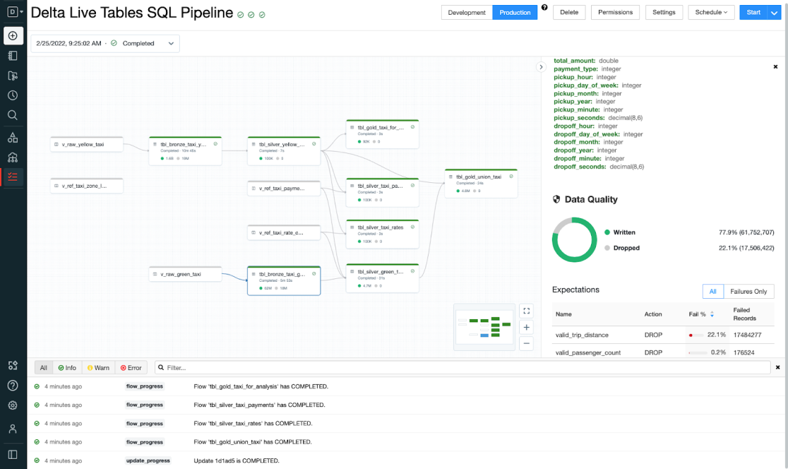 The UI of Delta Live Tables, Image source:
Databricks
The UI of Delta Live Tables, Image source:
Databricks
In addition, the display of the DAGs can also reload individual pipeline strings. This simplifies the handling significantly.
As mentioned above, you can also view information about the data quality directly in the graphs. This is possible with a click on the corresponding stage and is displayed in a nice sidebar. If you want to do even more visualization and also evaluate a longer time series of data quality tests, you can do this via Databricks SQL with a dashboard. Since the log information is stored in delta tables, it can be queried and visualized directly via SQL.
Conclusion
Now that I have told you a lot about Delta Live Tables, I would like to draw a conclusion. Of course, I have only touched on many things, but there are many more features that can be found in the documentation. But from my work with the framework, I can say that it simplifies many things and makes working with data pipelines much more pleasant than having to write them completely in code. Especially, the orchestration is extremely simple and possible with only a few lines of code.
The visualization of the data pipeline is also very well done and offers many possibilities for monitoring the data quality. If you do not already have a corresponding solution, DLT is a suitable alternative.
However, it is also a fact that one becomes somewhat dependent on the platform - much more so than was previously the case with Databricks. This is because the clusters are only available in managed form. Also, for the code there is only the notebook with the dlt package as the only usage option. The way back to Python or into a low-code alternative is therefore not so easy anymore.
Also, Databricks itself is already significantly more expensive than, say, Azure Mapping Dataflows or Azure Synapse Notebooks. With DLT, they step it up a notch, and if you want to use data quality testing, it gets even more expensive. So, for very long pipelines that run daily, it may be a good idea to go high code after all and run the pipeline on an inexpensive job cluster.
Finally, it remains to be said that DLT is not necessarily suitable for external extraction processes. For this, it is better to rely on separate jobs or use connectors as offered in low-code platforms, such as Azure Data Factory or AWS Glue. I rather intended DLT for data integration within a data lake. This means that, in reality, you have several solutions that work together more or less well.
DLT is therefore an excellent solution if you rely completely on Databricks and can or want to make yourself dependent on them. As a self-service solution with Databricks SQL and Databricks ML, it significantly simplifies the work with data pipelines.
However, if you don’t want to be tied down and fear the high costs, as well as the further overhead, then Delta Live Tables may not be the right solution. In the end, as always, it depends on the individual requirements, whether a new framework like DLT is worth it or not.
If you have any questions or feedback, feel free to write me a mail or reach out to me on any of my social media channels.